SVGs with LLMs.

An LLM can help you generate SVG drawings for the machines. This page walks through the workflow we recommend: a copy-paste setup, a way of describing what you want, and a few examples to try. No prior SVG or coding knowledge is needed.

LLMs are good at algorithmic drawings — patterns built from rules, math, or recursion. They are bad at drawings of things (“a flower,” “a face”). Treat the LLM like a collaborator for spirals, grids, fractals, and tilings — not as an illustrator. The skill you are learning is describing a system, not picturing a result.

1. Set up constraints once — paste the setup prompt below at the start of every new conversation.
2. Describe a system — tell the LLM what rule or structure to draw, not what the picture should look like.
3. Iterate in the Artifact — the SVG appears live next to the chat; refine through follow-up messages.

The setup prompt

Start every conversation by pasting this. It tells the LLM what kind of SVG to produce.

I'm making SVGs for a pen plotter. For everything in this conversation:
- Output as a single SVG artifact I can preview
- Stroke-only paths, no fills (fill="none")
- Single stroke width, 0.5mm
- Black strokes unless I specify otherwise
- viewBox in millimeters, sized for an A4 portrait page (210 x 297)
- 15mm margin from page edges
- No text elements, no raster images, no gradients, no opacity
- Use <path> elements where possible, with explicit d attributes

The LLM will acknowledge and then wait for your first drawing request.

There are infinitely many generative systems you can describe — different rules, different axioms, different interpretations. The four examples below were all produced by prompting an LLM. Each shows a preview, a downloadable SVG for the machine, and the recipe that produced it.

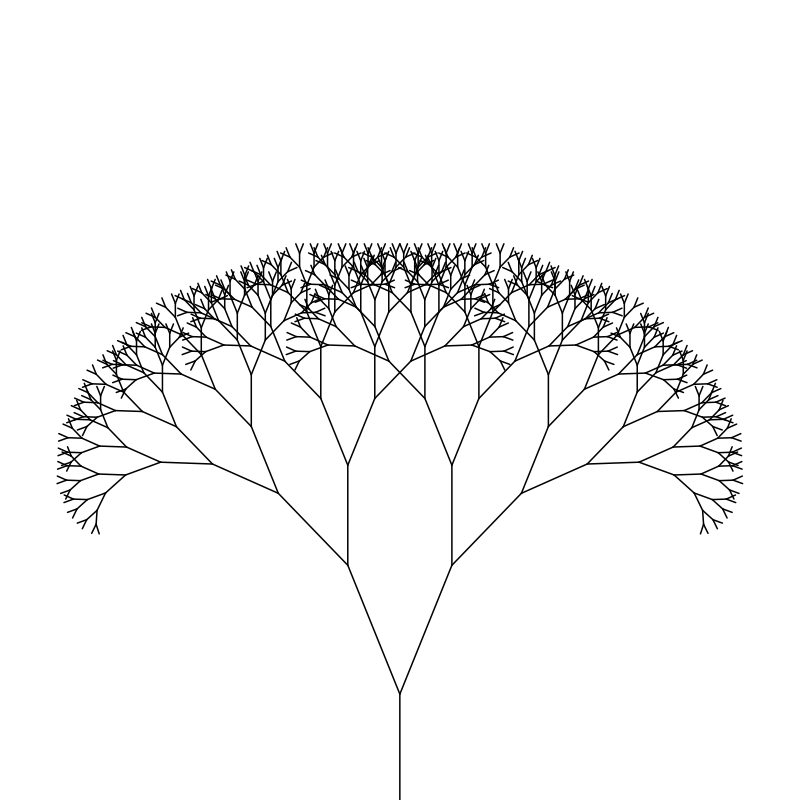
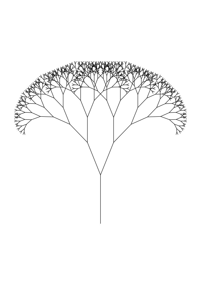
Binary fractal tree

Each branch splits into two children at a fixed angle, lengths shrink by a fixed ratio. Ten levels of recursion produce 1,024 branches from a single trunk.

Recipe

Branching rule: each branch splits into 2 children
Iterations: 10
Trunk length: 55mm
Split angle: 22° from parent direction
Length ratio per generation: 0.72

Download SVG

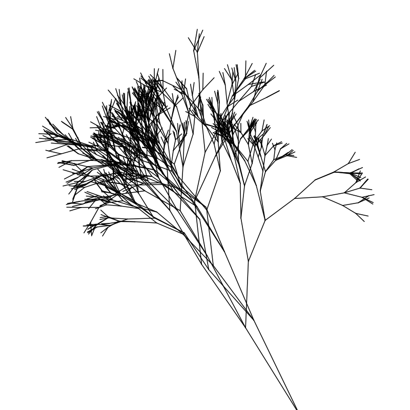
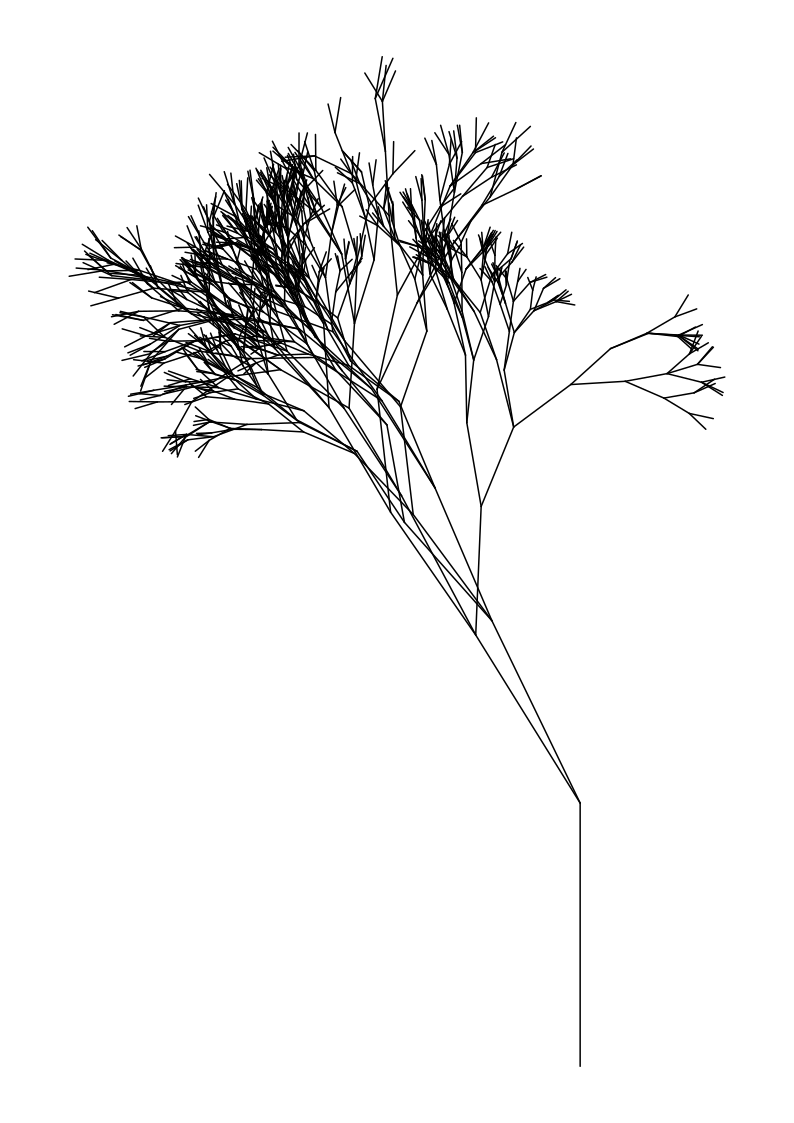
Stochastic tree

The same idea as the binary tree, but with randomness: angles and lengths jittered per branch, occasional three-way splits. The result feels less mathematical and more like a plant.

Recipe

Branching rule: 2 or 3 children (20% chance of 3)
Iterations: 9
Trunk length: 50mm
Split angle: 25° ± 12° (random per branch)
Length ratio: 0.74 ± 0.10 (random per branch)
Random seed: 7

Download SVG

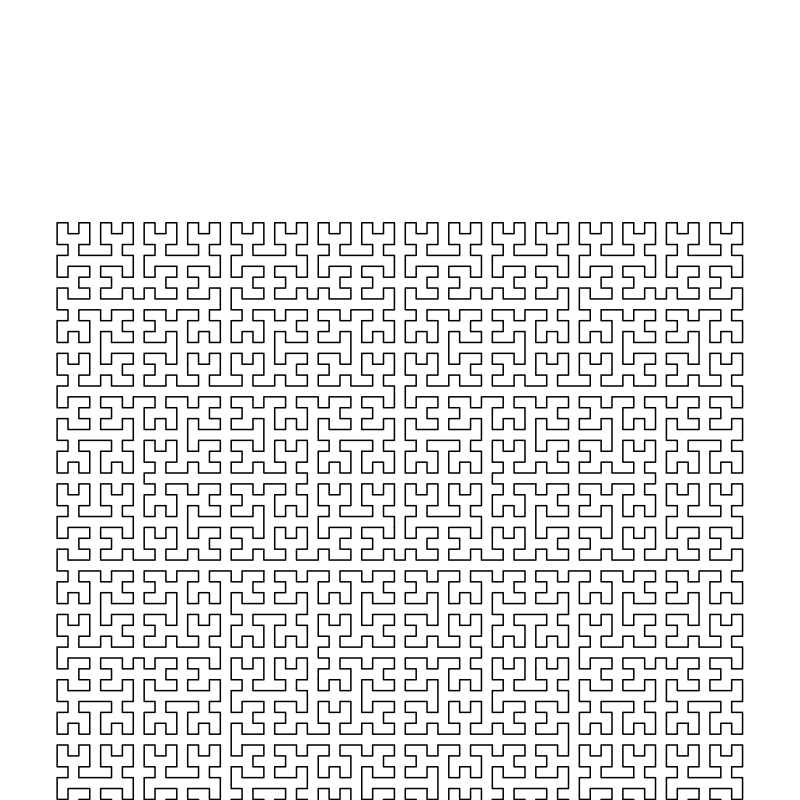
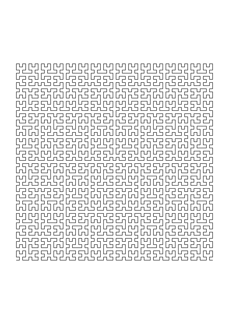
Hilbert curve

A space-filling curve drawn as one continuous line. 4,096 segments, zero pen-up travel between them — the most machine-efficient drawing on this page.

Recipe

L-system: Hilbert curve, order 6
Axiom: A
Rules: A → +BF-AFA-FB+, B → -AF+BFB+FA-
F = forward, + = turn left 90°, - = turn right 90°
Fills a square within the page margins

Download SVG

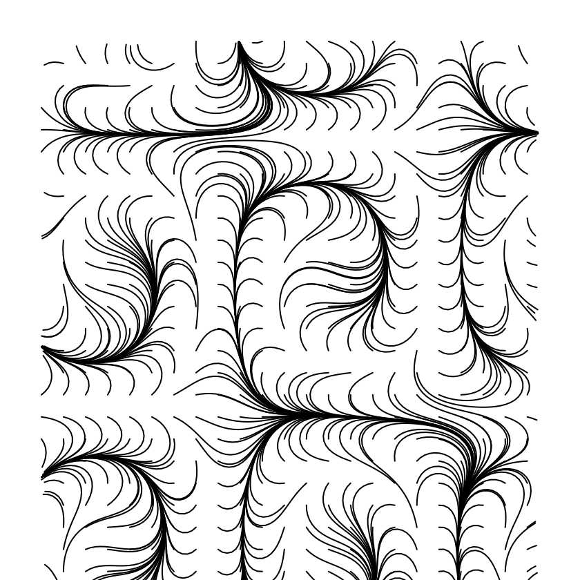
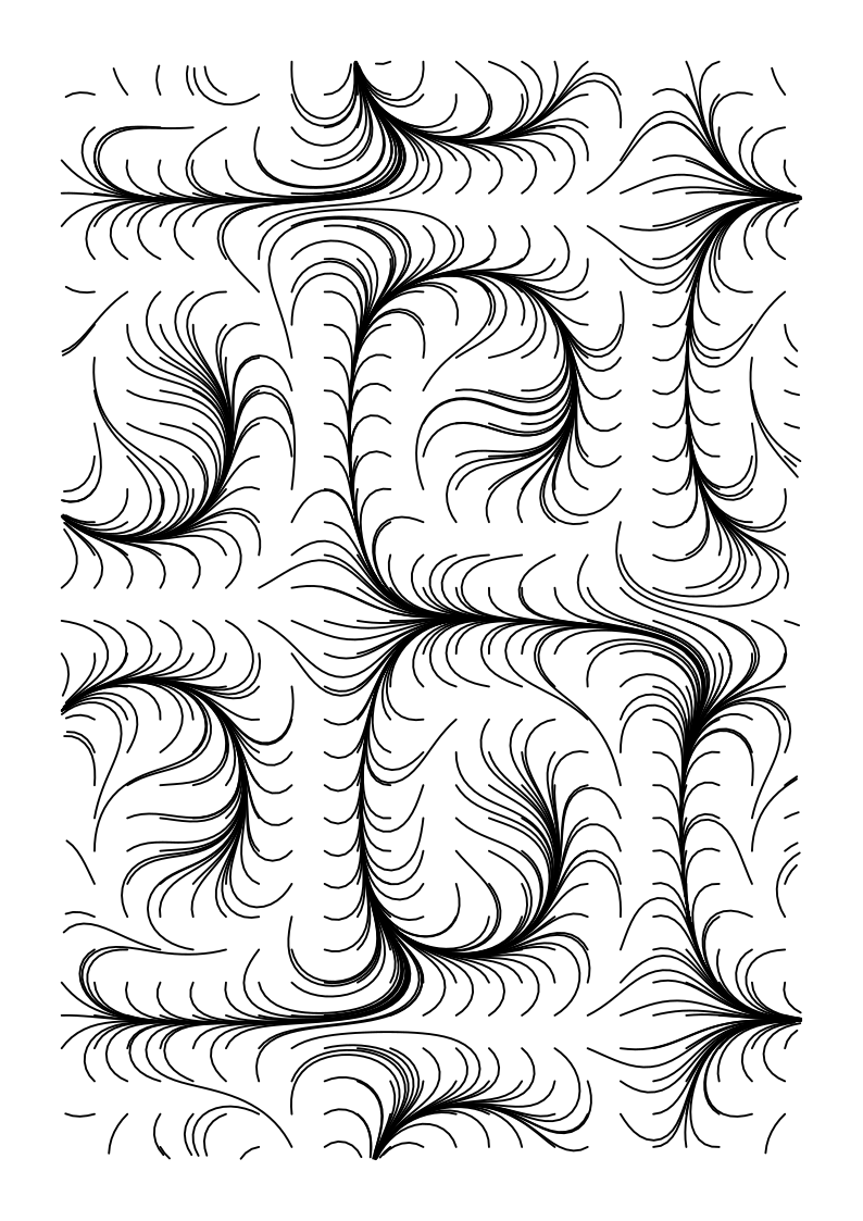
Flow field

737 streamlines traced through a trigonometric vector field. Each curve starts at a seed point and steps forward, turning according to the field at each position. Simple math, organic result.

Recipe

Seed grid: 23×34 points, 8mm spacing
Each streamline: up to 50 steps, 1.8mm per step
Angle at (x,y): sin(x·π/80) · cos(y·π/100) · 2π
  + 0.35·sin(r/30), r = distance from center
Streamlines stop at the 15mm page margin

Download SVG

These are not the only L-systems. Search for “Lindenmayer system” or “L-system gallery” online and you will find hundreds — Koch curves, dragon curves, Penrose tilings, ferns. Show the LLM one you like and ask for an SVG.

The biggest difference between getting useful results and frustrating ones is how you phrase the request. LLMs respond to rules, parameters, and structures much better than to adjectives or images. Three examples of the shift:

What to watch for

Math errors compound silently. LLMs make arithmetic mistakes, especially in dense parametric output. Always preview before plotting — don’t trust the SVG sight unseen.

The result can fall outside the page. Even with the setup prompt’s margins, scaling sometimes goes wrong. If your drawing looks clipped, ask the LLM to “scale this to fit within A4 portrait with 15mm margins.”

High density gets truncated. SVGs above roughly 2,000 line segments may cut off mid-output. If you want denser work, ask the LLM for the underlying Python or JavaScript code and run it yourself.

Screen-pretty isn’t machine-pretty. Fills, gradients, and very thin overlapping strokes look fine on a monitor but produce muddy or unplottable output. If something looks unexpectedly rich in the preview, ask: “Show me only the strokes that will actually be plotted.”

After the LLM, optimize. LLMs produce clean SVGs, but they don’t optimize them for machines. Pen-up travel, redundant segments, and path ordering all affect how long your drawing takes to plot — sometimes by an order of magnitude. Tools like vpype and Inkscape handle the optimization before you send to the machine.

Your first result is rarely the final one — and the LLM can take you well past anything the diagrams on this page can show. The Artifact updates each time you send a new message, so refinement is a conversation. A few phrasings that consistently work:

• “Increase the density to 800 points.”
• “Add a second layer rotated 30°.”
• “Center the composition vertically on the page.”
• “Reduce the stroke width to 0.3mm.”
• “Make every fifth element bolder.”
• “Remove elements where the radius exceeds 80mm.”

Change one variable at a time. If you change three things at once and don’t like the result, you won’t know which change to undo.

Phyllotaxis is the arrangement of seeds in a sunflower or petals on a stem: each new element is placed at a fixed angle (about 137.5°, the golden angle) from the last. It is one formula and one constant, and it produces the spiral structure you see throughout nature.

The prompt

Generate an SVG for a pen plotter following my constraints above.

Place 500 points in a Fibonacci phyllotaxis arrangement: each point i
is at radius r = c·√i and angle θ = i · 137.508°, centered on the page.
Choose c so the pattern fills the page within the 15mm margin.

Draw a small circle (radius 0.4mm at the center growing to 1mm at the
edge) at each point.

Same system, different prompts

Each option in the dropdown comes from one short follow-up message after the first prompt. The same points, connected by different rules:

“Spiral arms (13+21)” was produced by asking:

Instead of drawing circles, draw two families of spiral arms:
connect every 13th point with a polyline, and separately connect
every 21st point. (13 and 21 are consecutive Fibonacci numbers.)

“Spiral arms (21)” was produced by asking:

Instead of drawing circles, connect every 21st point with a polyline.

“Nearest neighbors” was produced by asking:

Instead of drawing circles, connect each point to its two nearest
neighbors with straight lines.

The takeaway

Same point set, different rules, different drawings. This is the core idea: you are not describing pictures — you are describing how the rules connect things together. Once you internalize this, you can describe systems the LLM has never seen before and get useful drawings back.

An L-system (Lindenmayer system) is a rewriting rule applied repeatedly to a string of symbols, then interpreted as drawing commands. A handful of characters and an angle produce remarkably plant-like structures. This is the kind of thing LLMs do well because the description is a system, not a picture.

The prompt

Generate an SVG for a pen plotter following my constraints above.

Draw an L-system fractal plant.
- Axiom: X
- Rules: X → F+[[X]-X]-F[-FX]+X, and F → FF
- Iterate the rules 4 times
- Turn angle: 25°
- Interpret the resulting string as turtle graphics: F = draw forward,
  + = turn right, - = turn left, [ = push state, ] = pop state, X = no draw
- Start at the bottom of the page pointing up
- Choose step length so the plant fills the lower two-thirds of the page
  with margin

Below are three starting prompts. Paste the setup prompt from above first, then any one of these. Then start iterating.

Draw a 20×20 grid of square cells (each 8mm). In each cell, draw one
diagonal line, chosen randomly between / and \. Connect adjacent
diagonals into continuous polylines where possible.

Draw 30 concentric circles centered on the page, with radii from 10mm
to 90mm in 2.5mm increments. Perturb the radius of each circle with
sine noise (amplitude 3mm, 7 cycles per revolution), with the noise
phase shifting by 11° between circles.

Draw a flow field: a 30×40 grid of short line segments (each 6mm long).
Each segment's angle is determined by the function θ(x,y) = sin(x/40)·cos(y/50)
multiplied by 2π. Center the field on the page.

If something breaks, that’s the lesson. Ask the LLM what went wrong, or just try again with one variable changed.